The most important element of any robot is the controller. The control algorithm determines how the robot should react to different sensor inputs, allowing it to intelligently adapt to and interact with its environment. Especially for a self-balancing robot, the control program is vital as it interprets the motion sensor data and decides how much the motors need to be moved in order for the robot to remain stable and upright. The most common controller used for stabilisation systems is the PID controller. So let’s look at how it works…
The PID Controller
PID stands for Proportional, Integral and Derivative, referring to the mathematical equations used to calculate the output of the controller. This is perhaps the most common type of controller used in industry, as it is able to control relatively complex systems even though the calculations are actually quite straightforward (making it easy to program and fast to compute). Mathematically, the PID controller can be described by the following formula:
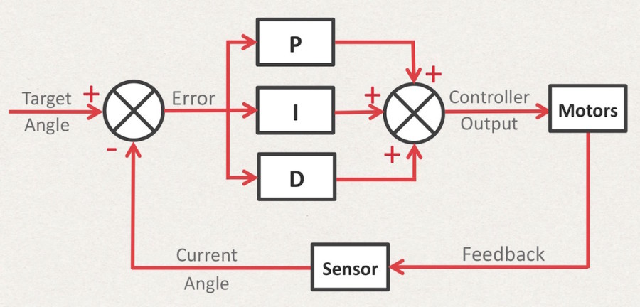
u(t)=K_pe(t) + K_i\int_{0}^{t}e(t)dt +K_d\frac{de(t)}{dt}In this formula, the output of the controller u(t) is determined by the sum of three different elements, each dependent on the error e(t). The error simply is the difference between the target value and the current value (measured by the sensor). Now let’s quickly look at what each of the terms in the equation is doing for our robot…
K_pe(t)
This is the proportional component, which takes the current error value and multiplies it by a constant number (Kp). For our self-balancing robot, this simply takes in the current angle of the robot and makes the motors move in the same direction as the robot is falling. The further the robot falls off target, the faster the motors move. If the P-component is used on its own, the robot might stabilise for a while, but the system will tend to overshoot, oscillate and ultimately fall over.
K_i\int_0^te(t)dt
The integral component is used to accumulate any errors over time, and multiplies this accumulated value by a constant number (Ki). For example if the robot tends to fall over to one side, it knows that it needs to move in the opposite direction in order to keep on target and to prevent drifting left or right.
K_d\frac{de(t)}{dt}Finally, the derivative component is responsible for dampening any oscillations and ensures that the robot does not overshoot the target value. Each time the controller is called, this term calculates the change in the error value and multiplies it by a constant number (Kd). Often this is simplified to calculate only the change in the current sensor value, rather than the change in error. If the target position remains constant, this gives the same result. This simplification helps to prevent sudden jumps in the output value which happen when the target position it changed.
Summing all three of these terms together then gives us an output value which we can send to the motor of the self-balancing robot. However, before the controller can successfully balance the robot, the three constants (Kp), (Ki) and (Kd) need to be tuned to suit our specific application. By increasing or decreasing the values of these constants, we control how much each of the three components of the controller contributes to the output of the system.
The formula I used above is called the “Independent” PID equation. If you read up on the PID controller online, you may also see the formula for the algorithm expressed in a different format (known as the “Dependent” PID equation):
u(t) = K_ce(t)+\frac{K_c}{T_i}\int_0^te(t)dt + K_cT_d\frac{de(t)}{dt}The term (Kc) is known as controller gain, (Ti) the integral time and (Td) the derivative time. This format can be useful when using some automated tuning techniques, however the final result is the same.
Implementing the Controller
Now that we know the basic theory, we can start to write this in code. The basic layout of the function is shown below. The controller can be used by calling the “pid” function at regular intervals, providing the target position and the current position (as recorded by the sensor) as parameters of the function. The function then outputs the calculated result of the controller. Tuning of the controller can be done by changing the values of the (Kp), (Ki) and (Kd) variables at the top of the code.
// Declare variables
float Kp = 7;          // (P)roportional Tuning Parameter
float Ki = 6;          // (I)ntegral Tuning Parameter
float Kd = 3;          // (D)erivative Tuning Parameter
float iTerm = 0;       // Used to accumulate error (integral)
float lastTime = 0;    // Records the time the function was last called
float maxPID = 255;    // The maximum value that can be output
float oldValue = 0;    // The last sensor value

/**
 * PID Controller
 * @param  (target)  The target position/value we are aiming for
 * @param  (current) The current value, as recorded by the sensor
 * @return The output of the controller
 */
float pid(float target, float current) {
	// Calculate the time since function was last called
	float thisTime = millis();
	float dT = thisTime - lastTime;
	lastTime = thisTime;

	// Calculate error between target and current values
	float error = target - current;

	// Calculate the integral term
	iTerm += error * dT;

	// Calculate the derivative term (using the simplification)
	float dTerm = (oldValue - current) / dT;

	// Set old variable to equal new ones
	oldValue = current;

	// Multiply each term by its constant, and add it all up
	float result = (error * Kp) + (iTerm * Ki) + (dTerm * Kd);

	// Limit PID value to maximum values
	if (result > maxPID) result = maxPID;
	else if (result < -maxPID) result = -maxPID;

	return result;
}
What does this program do?
First of all, the algorithm calculates the time since the last loop was called, using the “millis()” function. The error is then calculated; this is the difference between the current value (the angle recorded by the sensor), and the target value (the angle of 0 degrees we are aiming to reach).
The PID values are then calculated and summed up to give an output for the motors. The output is then constrained to ±255 as this is the maximum PWM value that can be output to the motors of the self-balancing robot.
Although this program is almost complete, I found that my robot only worked well once I included a timing function. This is a system that ensures the PID controller function is called at regular intervals. In my self-balancing robot, I set the loop time to be 10ms (meaning the function is run 100 times per second). Here is the timer code and a sample loop function:
// Any variables for the PID controller go here!
float targetValue = 0;

// Variables for Time Keeper function:
#define LOOP_TIME 10          // Time in ms (10ms = 100Hz)
unsigned long timerValue = 0;

/******** SETUP ************/
void setup() {
	// Put all of your setup code here
	timerValue = millis();
}

/******* MAIN LOOP *********/
void loop() {
	// Only run the controller once the time interval has passed
	if (millis() - timerValue > LOOP_TIME) {
		timerValue = millis();

		// Replace getAngle() with your sensor data reading
		float currentValue = getAngle();

		// Run the PID controller
		float motorOutput = pid(targetValue, currentValue);

		// Replace moveMotors() with your desired output
		moveMotors(motorOutput);
	}
}

/****** PID CONTROLLER *****/
float pid(float target, float current) {

	// PID code from above goes in here!
	return result;
}
Unfortunately this is not the end of the story! Although the PID controller code is complete, suitable PID constants still need to be found to tune the controller for your specific robot. These constants depend on things such as weight, motor speed and the shape of the robot, and therefore they can vary significantly from robot to robot. Here is a quick explanation of how you should go about calibrating your PID values:
Calibrating your PID Controller
- Create some way in which you can change the PID constant of your robot while it is running. One option is to use a potentiometer or some other analogue input to be able to increase or decrease the PID constant. I personally used the USB connection and the serial monitor to send new PID values. This is important as you can then see straight away how well the new PID values are working, and you won’t have to re-upload the code hundreds of times!
- Set all PID constants to zero. This is as good a place to start as any…
- Slowly increase the P-constant value. While you are doing this, hold the robot to make sure it doesn’t fall over and smash into a million pieces! You should increase the P-constant until the robot responds quickly to any tilting, and then just makes the robot overshoot in the other direction.
- Now increase the I-constant. This component is a bit tricky to get right. You should keep this relatively low, as it can accumulate errors very quickly. In theory, the robot should be able to stabilise with only the P and I constants set, but will oscillate a lot and ultimately fall over.
- Raise the D-constant. A lot. The derivative components works against any motion, so it helps to dampen any oscillations and reduce overshooting. I found that this constant has to be set significantly higher than the other two (x10 to x100 more) in order to have any effect. All the same, don’t set it too high, as it will reduce the robot’s ability to react to external forces (aka. being pushed around).
- Spend many fruitless hours slightly modifying the PID values. This is probably the longest part of the procedure, as there isn’t much of a method to it. You just have to increase and decrease the values until you reach that perfect sweet-spot for your robot!
Please leave a comment below if you have any questions or suggestions.
Updated: 23rd May 2019 – Reformatted post and improved the code snippets.
Updated: 1st June 2020 – Add PID equations and improved the descriptions.